Recursive Drawing
Overview
You can only get so far into mathematical art without mentioning fractals! As a review, a fractal is an image for which the same structure is evident at any level of resolution.
Perhaps the simplest fractals are created by the process of recursively drawing a particular pattern. Let's examine some of these deceptively simple-looking images. Be warned: the greater the recursive depth, the longer the code will take to execute!
The basic structure for each of these programs is very similar, so let's go over that first. You begin with a function that will compute any global variables and compute and any non-iterative components of the drawing. Let's call this mainFunction. In mainFunction, you call a second function- a sub-function. Let's call it drawingFunction. drawingFunction does the job of drawing your recursive structure, and takes as an input the number of recursions you want. Then, importantly, drawingFunction calls itself. The only difference is that it calls itself with one less iteration. Thus, with a simple call to mainFunction you can draw an entire fractal structure!
Note that the 'code' you see here is not really code at all. This is what we call pseudo-code. It shows us the structure of the program we want to write, but will not run because the details haven't been filled in.
function mainFunction (totalNumberOfIterations)
set variables
maybe draw something
drawingFunction(totalNumberOfIterations)
function drawingFunction(remainingIterations)
draw stuff
drawingFunction(remainingIterations-1)
end
end
Spinning Triangle
For this example, we again harness the power of rotation! We want to draw a triangle centered around the origin [0,0]. Since we know that the three points of an equilateral triangle are separated by 120 degrees, we can simply rotate our first point to get our second and third points. Then we simply draw lines between them using the plot command.
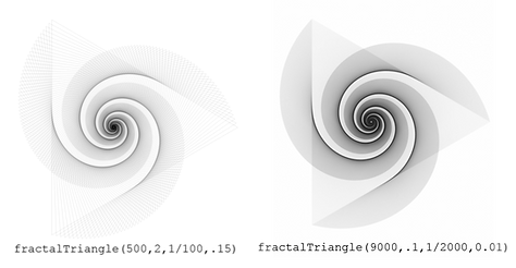
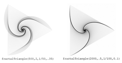
Okay, so now let's make this a fractal. We want to rotate the triangle with each iteration, and also shrink it slightly. So our draw subfunction will calculate the three points of the current triangle, based on the current length and angle parameters, and draw the triangle on top of the existing triangles. We should have something that looks like this:


function fractalTriangle(r,angleIncrement,lengthDecrement,transparency)
% Draw a fractal triangle, with the following inputs:
% r = int; number of iterations
% angleIncrement = number; amount the triangle rotates each iteration
% lengthDecrement = number; amount triangle shrinks each iteration
% transparency = number between 0 and 1; transparency of each triangle
figure('Position',[50,50,900,900],'Color',[1,1,1]);
drawTriangles(1,0,angleIncrement,r,r,lengthDecrement,transparency)
axis equal
axis off
function drawTriangles(len,angle,angInc,iterations,r,...
lengthDecrement,transparency)
% Draws the triangle for each iteration and calls itself. Inputs:
% len = number; length of a side of the triangle
% angle = number; amount the triangle rotates relative to previous
% iteration
% angleIncrement = number; amount the triangle rotates each iteration
% iterations = int; remaining number of iterations
% r = int; total number of iterations
% lengthDecrement = number; amount len changes each iteration
% transparency = number between 0 and 1; transparency of triangle
pt1x=len*cosd(angle);
pt1y=len*sind(angle);
rot=[cosd(120) -sind(120);sind(120) cosd(120)];
pt2=rot*[pt1x;pt1y];
pt3=rot*pt2;
c=[0 0 0];
p1=plot([pt1x,pt2(1),pt3(1),pt1x],[pt1y,pt2(2),pt3(2),pt1y],...
'Color',c,'LineWidth',3);
p1.Color(4)=transparency;
hold on
if iterations-1>0
drawTriangles(len-len*lengthDecrement,angle+angInc,...
angInc,iterations-1,r,lengthDecrement,transparency);
end
end
end
Basic Fractal Tree
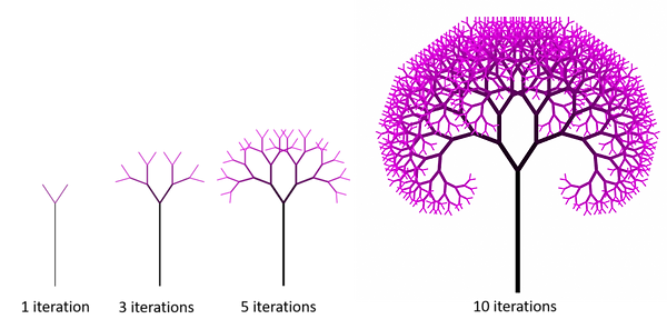
We'll continue with another 'simple' example: a branching tree. The recurring pattern is that every time you reach the end of a 'branch' in the tree, two more branches will fork out at equal angles. We want it to look something like the image below.

function fractalTreeBasic(r,angle,fade)
% This function draws a fractal tree with the following inputs:
% r = int; number of iterations
% angle = number; sideways angle of each of the two branches
% fade = 1 or 0; set value to 1 if you want branches to be transparent
totalIterations=r+1;
figure('Position',[10,10,900,900],'Color',[1,1,1]);
% Draw the tree trunk
c1=[0 0 0];len1=3*1.2^totalIterations;w1=r^0.6;
plot([0 0],[-len1,0],'LineWidth',w1,'Color',c1)
xlim([-2*len1,2*len1]);ylim([-2*len1,2*len1]);axis off; hold on;
% Begin the iterative process of drawing branches
drawBranches(90,[0,0],totalIterations-1,angle,totalIterations,fade);
function drawBranches(initAngle,pt,iterations,angle,totalIterations,fade)
% This sub-function draws the branches, recursively, with inputs:
% initAngle = number; the current angle of the 'trunk'
% pt = [x,y]; the endpoint of the 'trunk'
% iterations = number; number of times to repeat
% angle = number; amount each branch is splayed sideways
% The length of the current branch
len=1.2^(iterations);x1=pt(1);y1=pt(2);
ang1=initAngle+angle; % left branch angle
ang2=initAngle-angle; % right branch angle
% Use trigonometry to find the new branch endpoints
y2=len*sind(ang1)+y1;y3=len*sind(ang2)+y1;
x2=len*cosd(ang1)+x1;x3=len*cosd(ang2)+x1;
% Set the color based on the current iteration
c2=[1-iterations/(totalIterations) 0 1-iterations/(totalIterations)];
% Set the width of the branch based on the current iteration
w=iterations^0.6;
% Draw a line between the trunk and the left branch endpoint
p1=plot([x1,x2],[y1,y2],'LineWidth',w,'Color',c2);
% Draw a line between the trunk and the right branch endpoint
p2=plot([x1,x3],[y1,y3],'LineWidth',w,'Color',c2);
% Make the branches transparent if fade is set to 1
if fade==1
c4=1-(totalIterations-iterations)/totalIterations;
p1.Color(4)=c4;p2.Color(4)=c4;
end
% If you're not done iterating, draw branches at the end of each
% of the two branches you just created.
if iterations-1>0
drawBranches(ang1,[x2,y2],iterations-1,angle,totalIterations,fade);
drawBranches(ang2,[x3,y3],iterations-1,angle,totalIterations,fade);
end
end
end
Fractal Tree with Four Branches
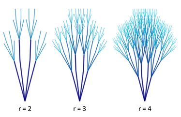
Okay, now let's take the fractal tree one step further. Instead of having two branches at every branch point, let's have 4. Thus, the first few iterations should look like this:

function fractalTreeFourBranches(r)
% This function draws a fractal tree with the following inputs:
% r = int; number of iterations
fig1=figure('Position',[50,50,1200,900],'Color',[1 1 1 1]);
drawBranch([0,0],90,r,r);
axis equal
axis off
function drawBranch(pt,angle,remainingIterations,r)
% This sub-function draws the branches, recursively, with inputs:
% angle = number; the current angle of the 'trunk'
% pt = [x,y]; the endpoint of the 'trunk'
% remainingIterations = number; number of times to repeat
% r = total number of iterations
% Scale the width and length by the number of iterations
width=5*(remainingIterations/r);
len1=5*remainingIterations;
ang1=angle+15;
ang2=angle+7;
ang3=angle-7;
ang4=angle-15;
% Use trig to figure out the new line endpoints
y1=len1*sind(ang1)+pt(2);
x1=len1*cosd(ang1)+pt(1);
y2=len1*sind(ang2)+pt(2);
x2=len1*cosd(ang2)+pt(1);
y3=len1*sind(ang3)+pt(2);
x3=len1*cosd(ang3)+pt(1);
y4=len1*sind(ang4)+pt(2);
x4=len1*cosd(ang4)+pt(1);
ang22=ang2-5;
ang33=ang3+5;
y22=len1/2*sind(ang22)+y2;
x22=len1/2*cosd(ang22)+x2;
y33=len1/2*sind(ang33)+y3;
x33=len1/2*cosd(ang33)+x3;
% Set the RGB color scaled by the current iteration
c=[0 1-(remainingIterations/r) 1-0.5*(remainingIterations/r)];
% Plot the four branches
p1=plot([pt(1),x1],[pt(2),y1],'LineWidth',width,'Color',c);
hold on
p2=plot([pt(1),x2],[pt(2),y2],'LineWidth',width,'Color',c);
p3=plot([pt(1),x3],[pt(2),y3],'LineWidth',width,'Color',c);
p4=plot([pt(1),x4],[pt(2),y4],'LineWidth',width,'Color',c);
p5=plot([x2,x22],[y2,y22],'LineWidth',width,'Color',c);
p6=plot([x3,x33],[y3,y33],'LineWidth',width,'Color',c);
% Set the branches to be slightly transparent
p1.Color(4)=0.8;
p2.Color(4)=0.8;
p3.Color(4)=0.8;
p4.Color(4)=0.8;
p5.Color(4)=0.8;
p6.Color(4)=0.8;
% Iterate; draw a new tree at each of the four branches
if remainingIterations-1>0
drawBranch([x1,y1],ang1,remainingIterations-1,r);
drawBranch([x22,y22],ang22,remainingIterations-1,r);
drawBranch([x33,y33],ang33,remainingIterations-1,r);
drawBranch([x4,y4],ang4,remainingIterations-1,r);
end
end
end
Fractal Fern
This example is meant to show you one of the really neat, remarkably realistic-looking things you can create with recursive drawing! We probably won't have the time to go over this in class, but of course feel free to play around with the code and let me know if you have any questions!
Also, please note that although it looks extremely similar, this is not a Barnsley Fern. The Barnsley Fern is also a fractal, but it is generated by a very different process. I encourage you to check it out if fractal leaves intrigue you!
Note the fractal structure of the leaf. That is, each frond of the fern itself looks like a fern! Okay, so in our drawing function we want to recursively draw the fern. Sounds simple enough so far, right?
Well there's a couple of factors that make it more complicated. The orientation of the fronds alternate right and left, and the curvature of those fronds depends on the direction. So we'll have to incorporate a variable that changes direction with every iteration.


function fractalFern(r)
% Draws a fractal fern with r iterations
% Initialize the figure
fig1=figure('Position',[50,50,750,900],'Color',[1 1 1]);
drawFern([0,0],r,1,90,10,r)
axis off
function drawFern(pt,numBranches,dir,initAng,length1,r)
% Draws each frond of the fern, taking inputs:
% pt = [x,y]; the endpoint of the current stem
% numBranches = int; number of branches to draw on the current frond
% dir = 1 or 0; determines the curvature of the frond
% initAng = number; the initial angle of the stem
% length1 = number; length of the first segment of the stem
% r = int; total number of stem segments
index=numBranches;
ang=initAng;
x2=pt(1);
y2=pt(2);
next=1;
% This while loop draws a new frond after drawing each stem
% segment, alternating left and right
while index>0
len=length1*.9^(numBranches-index);
% This simply stops the drawing if the length of the line
% becomes too small
if len<.05
return
end
% next determines the direction of the next frond; this code
% switches it every iteration
if next==1
next=0;
nextAng=ang-50;
else
next=1;
nextAng=ang+50;
end
% dir controls the direction of curvature of the stem
if dir==1
ang=ang-2;
else
ang=ang+2;
end
% calculate the endpoint of the current stem segment
xdraw=len*cosd(ang)+x2;
ydraw=len*sind(ang)+y2;
% determine the color of the current stem segment
c=[0, 1-(.7*(index/r)), 0];
% draw the current segment of the stem
plot([x2,xdraw],[y2,ydraw],'Color',c,'LineWidth',len/2);
hold on
x2=xdraw;
y2=ydraw;
% draw the next frond. Note that the number of branches
% to draw on each successive frond decreases by 1
drawFern([x2,y2],index-1,next,nextAng,len/2.5,r);
index=index-1;
end
end
end